In recent years, data science has become a huge attractive field with the profession of data scientist topping the list of the best jobs in America. And with all the hype that the field produces, one might ask: what does it take do be a data scientist?

Well… that’s a good question. First of all, there are a lot of requirements. But one of the most important ones is to learn how to work with data sets. And I am not talking about playing with spreadsheets. I am talking about working with some real programming language to get the job done with any datasets, no matter how huge it is.

Hence, this post is the first part of a series about working with tabular data with the Julia programming language. Of course, the aim of this post is not only to give you a quick introduction to the language, but also present to you how you can easily install and work rightaway with datasets with Julia.

Why Julia?

Glad you asked! Julia is a high level programming language released in 2012 by a team of MIT researchers. Since its beginning, the aim was to solve the so called two-language programing problem: easy to use functionalities of interpretable languages (Python, R, Matlab) vs high performance of compiled languages (C, C++, Fortran). According to its creators:

We want a language that’s open source, with a liberal license. We want the speed of C with the dynamism of Ruby. We want a language that’s homoiconic, with true macros like Lisp, but with obvious, familiar mathematical notation like Matlab. We want something as usable for general programming as Python, as easy for statistics as R, as natural for string processing as Perl, as powerful for linear algebra as Matlab, as good at gluing programs together as the shell. Something that is dirt simple to learn, yet keeps the most serious hackers happy. We want it interactive and we want it compiled. — julialang.org

Hence, Julia was born. Combining the JIT (Just In Time) compiler and Julia’s multiple-dispatch system plus the fact that its codebase is written entirely in native language, Julia gives birth to the popular phrase in the community:

“Walks like Python, runs like C.”

Installing Julia

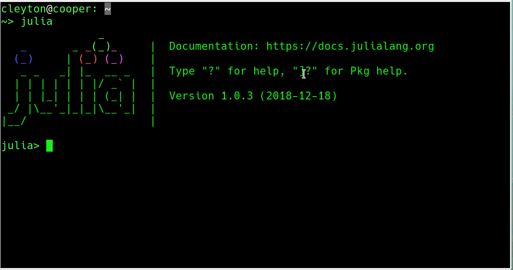
To play around with Julia there are some options. One obvious way is to download the official binaries from the site for your specific plataform (Windows, macOS, Linux, etc). At the time of this writting, the Current stable release is v1.1.0 and the Long-term support release is v1.0.3. Once you downloaded and execute the binaries, you will see the following window:

Another options is to use Julia in the browser on JuliaBox.com with Jupyter notebooks. No installation is required – just point your browser there, login and start playing around.

Installing Packages

All the package management in Julia is performed by the Pkg package. To install a given package we use Pkg.add("package_name"). In this tutorial we are going to use some packages that are not pre-installed with Julia. To install them, do the following:

using Pkg
Pkg.add("DataFrames")
Pkg.add("DataFramesMeta")
Pkg.add("CSV")

We installed three packages: DataFrames (which is the subject of this post), DataFramesMeta (we will use some of its functionalities) and CSV (to read and write CSV files).

Of course there is more about package management in Julia than I just showed. A great introduction is presented in this video by Jane Harriman. For more advanced usage, please refer to the official documentation.

Introduction to DataFrames in Julia

In Julia, tablular data is handled using the DataFrames package. Other packages are commonly used to read/write data into/from Julia such as CSV.

A data frame is created using the DataFrame() function:

using DataFrames 
foo = DataFrame();
foo

## 0×0 DataFrame

To use the functionalities of the package, let’s create some random data. I will use the rand() function to generate random numbers to create an array 100 x 10 and convert it to a data frame:

foo = DataFrame(rand(100, 10));
foo

## 100×10 DataFrame. Omitted printing of 4 columns
## │ Row │ x1         │ x2       │ x3        │ x4       │ x5        │ x6       │
## │     │ Float64    │ Float64  │ Float64   │ Float64  │ Float64   │ Float64  │
## ├─────┼────────────┼──────────┼───────────┼──────────┼───────────┼──────────┤
## │ 1   │ 0.0193136  │ 0.466228 │ 0.790475  │ 0.805074 │ 0.51182   │ 0.201707 │
## │ 2   │ 0.986082   │ 0.33719  │ 0.309992  │ 0.117098 │ 0.792606  │ 0.102682 │
## │ 3   │ 0.00366356 │ 0.323071 │ 0.685271  │ 0.596414 │ 0.847368  │ 0.105035 │
## │ 4   │ 0.297846   │ 0.136907 │ 0.726739  │ 0.569452 │ 0.922995  │ 0.846519 │
## │ 5   │ 0.73245    │ 0.208294 │ 0.353801  │ 0.448741 │ 0.185897  │ 0.496741 │
## │ 6   │ 0.209719   │ 0.114021 │ 0.0662264 │ 0.463682 │ 0.628582  │ 0.130653 │
## │ 7   │ 0.341692   │ 0.608349 │ 0.946541  │ 0.589161 │ 0.418321  │ 0.295541 │
## ⋮
## │ 93  │ 0.714495   │ 0.661317 │ 0.954527  │ 0.209581 │ 0.107941  │ 0.233787 │
## │ 94  │ 0.680497   │ 0.101874 │ 0.872371  │ 0.596457 │ 0.669133  │ 0.740674 │
## │ 95  │ 0.909319   │ 0.182776 │ 0.343387  │ 0.142707 │ 0.0140866 │ 0.791679 │
## │ 96  │ 0.642578   │ 0.949993 │ 0.380511  │ 0.96358  │ 0.878766  │ 0.270409 │
## │ 97  │ 0.605148   │ 0.240233 │ 0.144059  │ 0.545245 │ 0.0463105 │ 0.188397 │
## │ 98  │ 0.0907523  │ 0.334278 │ 0.288403  │ 0.519876 │ 0.267965  │ 0.552448 │
## │ 99  │ 0.751681   │ 0.289301 │ 0.488135  │ 0.382877 │ 0.320208  │ 0.999445 │
## │ 100 │ 0.856248   │ 0.577105 │ 0.588476  │ 0.435958 │ 0.0163749 │ 0.337817 │

Maybe you have noticed the “;” at the end of a command. It turns out that in Julia, contrary to many other languages, everything is an expression, so it will return a result. Hence, to turn off this return, we must include the “;” at the end of each command.

To get the dimension of a data frame, we can use the size() function. Also, similarly to R programming language, nrow() and ncol() are available to get the number of rows and columns, respectively:

size(foo)

## (100, 10)

nrow(foo)

## 100

ncol(foo)

## 10

Another basic task when working with datasets is to to get the names of each variable contained in the table. We use the names() function to get the column names:

names(foo)

## 10-element Array{Symbol,1}:
##  :x1 
##  :x2 
##  :x3 
##  :x4 
##  :x5 
##  :x6 
##  :x7 
##  :x8 
##  :x9 
##  :x10

To get a summary of the dataset in general, we can use the function describe():

describe(foo)

## 10×8 DataFrame. Omitted printing of 2 columns
## │ Row │ variable │ mean     │ min        │ median   │ max      │ nunique │
## │     │ Symbol   │ Float64  │ Float64    │ Float64  │ Float64  │ Nothing │
## ├─────┼──────────┼──────────┼────────────┼──────────┼──────────┼─────────┤
## │ 1   │ x1       │ 0.502457 │ 0.00190391 │ 0.508102 │ 0.993014 │         │
## │ 2   │ x2       │ 0.461593 │ 0.0143797  │ 0.465052 │ 0.949993 │         │
## │ 3   │ x3       │ 0.4659   │ 0.0180212  │ 0.409124 │ 0.978917 │         │
## │ 4   │ x4       │ 0.503142 │ 0.0130052  │ 0.508707 │ 0.986293 │         │
## │ 5   │ x5       │ 0.518394 │ 0.00177395 │ 0.502389 │ 0.994104 │         │
## │ 6   │ x6       │ 0.486075 │ 0.00543681 │ 0.475648 │ 0.999445 │         │
## │ 7   │ x7       │ 0.490961 │ 0.00366989 │ 0.482302 │ 0.996092 │         │
## │ 8   │ x8       │ 0.503405 │ 0.0180501  │ 0.525201 │ 0.985918 │         │
## │ 9   │ x9       │ 0.507343 │ 0.0327247  │ 0.533176 │ 0.990731 │         │
## │ 10  │ x10      │ 0.468541 │ 0.00622055 │ 0.470003 │ 0.996703 │         │

Note that there is a message indicating the omission of some columns. This is the default behavior of Julia. To avoid this feature, we use the show() function as follows:

show(describe(foo), allcols = true)

Manipulating Rows:

Subset rows in Julia can be a little odd in the beginning, but once you get used to, it becomes more logical. For example, suppose we want the rows where x1 is above its average. We could this as follows:

## Loading the Statistics package:
using Statistics
## Creating the conditional:
cond01 = foo[:x1] .>= mean(foo[:x1]);
## Subsetting the rows:
foo[cond01, :]

## 51×10 DataFrame. Omitted printing of 4 columns
## │ Row │ x1       │ x2       │ x3        │ x4       │ x5        │ x6        │
## │     │ Float64  │ Float64  │ Float64   │ Float64  │ Float64   │ Float64   │
## ├─────┼──────────┼──────────┼───────────┼──────────┼───────────┼───────────┤
## │ 1   │ 0.986082 │ 0.33719  │ 0.309992  │ 0.117098 │ 0.792606  │ 0.102682  │
## │ 2   │ 0.73245  │ 0.208294 │ 0.353801  │ 0.448741 │ 0.185897  │ 0.496741  │
## │ 3   │ 0.716057 │ 0.325789 │ 0.193415  │ 0.813209 │ 0.232703  │ 0.314502  │
## │ 4   │ 0.538082 │ 0.932279 │ 0.101212  │ 0.363205 │ 0.979265  │ 0.274936  │
## │ 5   │ 0.693567 │ 0.78976  │ 0.123106  │ 0.566847 │ 0.492958  │ 0.798202  │
## │ 6   │ 0.794447 │ 0.405418 │ 0.0521367 │ 0.587886 │ 0.922298  │ 0.211156  │
## │ 7   │ 0.664186 │ 0.432662 │ 0.0431839 │ 0.810072 │ 0.963643  │ 0.678182  │
## ⋮
## │ 44  │ 0.85821  │ 0.484308 │ 0.899559  │ 0.754818 │ 0.252699  │ 0.0590497 │
## │ 45  │ 0.714495 │ 0.661317 │ 0.954527  │ 0.209581 │ 0.107941  │ 0.233787  │
## │ 46  │ 0.680497 │ 0.101874 │ 0.872371  │ 0.596457 │ 0.669133  │ 0.740674  │
## │ 47  │ 0.909319 │ 0.182776 │ 0.343387  │ 0.142707 │ 0.0140866 │ 0.791679  │
## │ 48  │ 0.642578 │ 0.949993 │ 0.380511  │ 0.96358  │ 0.878766  │ 0.270409  │
## │ 49  │ 0.605148 │ 0.240233 │ 0.144059  │ 0.545245 │ 0.0463105 │ 0.188397  │
## │ 50  │ 0.751681 │ 0.289301 │ 0.488135  │ 0.382877 │ 0.320208  │ 0.999445  │
## │ 51  │ 0.856248 │ 0.577105 │ 0.588476  │ 0.435958 │ 0.0163749 │ 0.337817  │

What if we want two conditionals? For example, we want the same condition as before and/or the rows where x2 is greater than or equal its average? Now things become trickier. Let’s check how we could do this:

## Creating the second conditional:
cond02 = foo[:x2] .>= mean(foo[:x2]);
## Subsetting cond01 AND cond02:
foo[.&(cond01, cond02), :]

## 25×10 DataFrame. Omitted printing of 4 columns
## │ Row │ x1       │ x2       │ x3        │ x4        │ x5        │ x6        │
## │     │ Float64  │ Float64  │ Float64   │ Float64   │ Float64   │ Float64   │
## ├─────┼──────────┼──────────┼───────────┼───────────┼───────────┼───────────┤
## │ 1   │ 0.538082 │ 0.932279 │ 0.101212  │ 0.363205  │ 0.979265  │ 0.274936  │
## │ 2   │ 0.693567 │ 0.78976  │ 0.123106  │ 0.566847  │ 0.492958  │ 0.798202  │
## │ 3   │ 0.567098 │ 0.747233 │ 0.589314  │ 0.0677154 │ 0.630238  │ 0.357654  │
## │ 4   │ 0.976991 │ 0.648552 │ 0.32794   │ 0.36951   │ 0.846276  │ 0.117798  │
## │ 5   │ 0.553247 │ 0.615375 │ 0.122955  │ 0.440636  │ 0.283713  │ 0.734161  │
## │ 6   │ 0.849795 │ 0.703195 │ 0.232944  │ 0.668432  │ 0.686921  │ 0.788872  │
## │ 7   │ 0.530801 │ 0.825475 │ 0.644381  │ 0.15488   │ 0.669306  │ 0.151317  │
## ⋮
## │ 18  │ 0.665926 │ 0.943121 │ 0.438038  │ 0.921251  │ 0.82234   │ 0.761529  │
## │ 19  │ 0.987506 │ 0.946972 │ 0.0462434 │ 0.67867   │ 0.731762  │ 0.482322  │
## │ 20  │ 0.862284 │ 0.886346 │ 0.694874  │ 0.0166389 │ 0.386215  │ 0.527352  │
## │ 21  │ 0.855198 │ 0.650342 │ 0.0321678 │ 0.723076  │ 0.449779  │ 0.0364525 │
## │ 22  │ 0.85821  │ 0.484308 │ 0.899559  │ 0.754818  │ 0.252699  │ 0.0590497 │
## │ 23  │ 0.714495 │ 0.661317 │ 0.954527  │ 0.209581  │ 0.107941  │ 0.233787  │
## │ 24  │ 0.642578 │ 0.949993 │ 0.380511  │ 0.96358   │ 0.878766  │ 0.270409  │
## │ 25  │ 0.856248 │ 0.577105 │ 0.588476  │ 0.435958  │ 0.0163749 │ 0.337817  │

## Subsetting cond01 OR cond02:
foo[.|(cond01, cond02), :]

## 77×10 DataFrame. Omitted printing of 4 columns
## │ Row │ x1        │ x2       │ x3        │ x4       │ x5        │ x6        │
## │     │ Float64   │ Float64  │ Float64   │ Float64  │ Float64   │ Float64   │
## ├─────┼───────────┼──────────┼───────────┼──────────┼───────────┼───────────┤
## │ 1   │ 0.0193136 │ 0.466228 │ 0.790475  │ 0.805074 │ 0.51182   │ 0.201707  │
## │ 2   │ 0.986082  │ 0.33719  │ 0.309992  │ 0.117098 │ 0.792606  │ 0.102682  │
## │ 3   │ 0.73245   │ 0.208294 │ 0.353801  │ 0.448741 │ 0.185897  │ 0.496741  │
## │ 4   │ 0.341692  │ 0.608349 │ 0.946541  │ 0.589161 │ 0.418321  │ 0.295541  │
## │ 5   │ 0.413762  │ 0.644062 │ 0.495503  │ 0.96149  │ 0.249137  │ 0.592854  │
## │ 6   │ 0.129374  │ 0.663032 │ 0.0180212 │ 0.280431 │ 0.887136  │ 0.329406  │
## │ 7   │ 0.716057  │ 0.325789 │ 0.193415  │ 0.813209 │ 0.232703  │ 0.314502  │
## ⋮
## │ 70  │ 0.85821   │ 0.484308 │ 0.899559  │ 0.754818 │ 0.252699  │ 0.0590497 │
## │ 71  │ 0.714495  │ 0.661317 │ 0.954527  │ 0.209581 │ 0.107941  │ 0.233787  │
## │ 72  │ 0.680497  │ 0.101874 │ 0.872371  │ 0.596457 │ 0.669133  │ 0.740674  │
## │ 73  │ 0.909319  │ 0.182776 │ 0.343387  │ 0.142707 │ 0.0140866 │ 0.791679  │
## │ 74  │ 0.642578  │ 0.949993 │ 0.380511  │ 0.96358  │ 0.878766  │ 0.270409  │
## │ 75  │ 0.605148  │ 0.240233 │ 0.144059  │ 0.545245 │ 0.0463105 │ 0.188397  │
## │ 76  │ 0.751681  │ 0.289301 │ 0.488135  │ 0.382877 │ 0.320208  │ 0.999445  │
## │ 77  │ 0.856248  │ 0.577105 │ 0.588476  │ 0.435958 │ 0.0163749 │ 0.337817  │

In Julia, instead of the syntax condition1 & condition2, which is more common in other programming languages, we use &(condition1, condition2) or |(condition1, condition2) operators to perform multiple conditional filtering.

Now, let’s say you have a DataFrame and you want to append rows to it. There are a couple of ways of doing data. The first one is to use the [data1; data2] syntax:

## Creating a DataFrame with 3 rows and 5 columns:
x = DataFrame(rand(3, 5));
## Let's add another line using [dataset1; dataset2] syntax:
[ x ; DataFrame(rand(1, 5)) ]

## 4×5 DataFrame
## │ Row │ x1       │ x2        │ x3        │ x4       │ x5        │
## │     │ Float64  │ Float64   │ Float64   │ Float64  │ Float64   │
## ├─────┼──────────┼───────────┼───────────┼──────────┼───────────┤
## │ 1   │ 0.722487 │ 0.0930212 │ 0.146     │ 0.486439 │ 0.0892853 │
## │ 2   │ 0.640469 │ 0.5902    │ 0.667832  │ 0.882527 │ 0.766987  │
## │ 3   │ 0.094589 │ 0.805257  │ 0.291809  │ 0.582878 │ 0.704144  │
## │ 4   │ 0.18066  │ 0.187027  │ 0.0440521 │ 0.077637 │ 0.884914  │

We could get the same result using the vcat() function. According to the documentation, vcat() performs concatenation along dimension 1, which means it will concatenate rows. The syntax would be:

## taking the first 2 lines and append with the third one:
vcat(x[1:2, :] , x[3, :])

Another way to do that is using the function append!(). This function will append a new row to the last row in a given DataFrame. Note that the column names must match exactly.

## Column names matches
append!(x, DataFrame(rand(1, 5)))

## 4×5 DataFrame
## │ Row │ x1       │ x2        │ x3        │ x4       │ x5        │
## │     │ Float64  │ Float64   │ Float64   │ Float64  │ Float64   │
## ├─────┼──────────┼───────────┼───────────┼──────────┼───────────┤
## │ 1   │ 0.722487 │ 0.0930212 │ 0.146     │ 0.486439 │ 0.0892853 │
## │ 2   │ 0.640469 │ 0.5902    │ 0.667832  │ 0.882527 │ 0.766987  │
## │ 3   │ 0.094589 │ 0.805257  │ 0.291809  │ 0.582878 │ 0.704144  │
## │ 4   │ 0.492341 │ 0.823765  │ 0.0731187 │ 0.123074 │ 0.264452  │

Note that if the column names between two DataFrames do not match , the append!() function is going to throw an error. Although this kind of behavior is important when we want to control for possible side effects, we might also prefer to not worry about this and “force” the append procedure. In order to do this we can make use of the push!() function.

## providing an Array:
push!(x, rand(ncol(x)))

## 5×5 DataFrame
## │ Row │ x1       │ x2        │ x3        │ x4       │ x5        │
## │     │ Float64  │ Float64   │ Float64   │ Float64  │ Float64   │
## ├─────┼──────────┼───────────┼───────────┼──────────┼───────────┤
## │ 1   │ 0.722487 │ 0.0930212 │ 0.146     │ 0.486439 │ 0.0892853 │
## │ 2   │ 0.640469 │ 0.5902    │ 0.667832  │ 0.882527 │ 0.766987  │
## │ 3   │ 0.094589 │ 0.805257  │ 0.291809  │ 0.582878 │ 0.704144  │
## │ 4   │ 0.492341 │ 0.823765  │ 0.0731187 │ 0.123074 │ 0.264452  │
## │ 5   │ 0.632829 │ 0.357564  │ 0.09631   │ 0.198201 │ 0.924137  │

## providing an dictionary:
push!(x, Dict(:x1 => rand(),
              :x2 => rand(),
              :x3 => rand(),
              :x4 => rand(),
              :x5 => rand()))

## 6×5 DataFrame
## │ Row │ x1       │ x2        │ x3        │ x4       │ x5        │
## │     │ Float64  │ Float64   │ Float64   │ Float64  │ Float64   │
## ├─────┼──────────┼───────────┼───────────┼──────────┼───────────┤
## │ 1   │ 0.722487 │ 0.0930212 │ 0.146     │ 0.486439 │ 0.0892853 │
## │ 2   │ 0.640469 │ 0.5902    │ 0.667832  │ 0.882527 │ 0.766987  │
## │ 3   │ 0.094589 │ 0.805257  │ 0.291809  │ 0.582878 │ 0.704144  │
## │ 4   │ 0.492341 │ 0.823765  │ 0.0731187 │ 0.123074 │ 0.264452  │
## │ 5   │ 0.632829 │ 0.357564  │ 0.09631   │ 0.198201 │ 0.924137  │
## │ 6   │ 0.234059 │ 0.530488  │ 0.0448796 │ 0.565734 │ 0.262909  │

As we can see, this function also accepts that we give a dictionary or an array to append to a DataFrame.

So, there are at least 4 methods to add rows to a DataFrame. Which one to use? Let’s see how fast it is each function:

using BenchmarkTools
@btime [x ; DataFrame(rand(1, 5))];
@btime vcat(x, DataFrame(rand(1, 5)));
@btime append!(x, DataFrame(rand(1, 5)));
@btime push!(x, rand(1, 5));

Manipulating Columns:

One of the first things we would want to do when working with a dataset is selecting some columns. In Julia, the syntax of selecting columns in DataFrames is similar to the one used in Matlab/Octave. For instance, we can make use of the “:” symbol to represent that we want all columns (or all rows) and/or a sequence of them:

## Taking all rows of the first 2 columns:
foo[:, 1:2]

## 100×2 DataFrame
## │ Row │ x1         │ x2       │
## │     │ Float64    │ Float64  │
## ├─────┼────────────┼──────────┤
## │ 1   │ 0.0193136  │ 0.466228 │
## │ 2   │ 0.986082   │ 0.33719  │
## │ 3   │ 0.00366356 │ 0.323071 │
## │ 4   │ 0.297846   │ 0.136907 │
## │ 5   │ 0.73245    │ 0.208294 │
## │ 6   │ 0.209719   │ 0.114021 │
## │ 7   │ 0.341692   │ 0.608349 │
## ⋮
## │ 93  │ 0.714495   │ 0.661317 │
## │ 94  │ 0.680497   │ 0.101874 │
## │ 95  │ 0.909319   │ 0.182776 │
## │ 96  │ 0.642578   │ 0.949993 │
## │ 97  │ 0.605148   │ 0.240233 │
## │ 98  │ 0.0907523  │ 0.334278 │
## │ 99  │ 0.751681   │ 0.289301 │
## │ 100 │ 0.856248   │ 0.577105 │

## Taking the first 10 rows of all columns:
foo[1:10, :]

## 10×10 DataFrame. Omitted printing of 4 columns
## │ Row │ x1         │ x2       │ x3        │ x4       │ x5       │ x6       │
## │     │ Float64    │ Float64  │ Float64   │ Float64  │ Float64  │ Float64  │
## ├─────┼────────────┼──────────┼───────────┼──────────┼──────────┼──────────┤
## │ 1   │ 0.0193136  │ 0.466228 │ 0.790475  │ 0.805074 │ 0.51182  │ 0.201707 │
## │ 2   │ 0.986082   │ 0.33719  │ 0.309992  │ 0.117098 │ 0.792606 │ 0.102682 │
## │ 3   │ 0.00366356 │ 0.323071 │ 0.685271  │ 0.596414 │ 0.847368 │ 0.105035 │
## │ 4   │ 0.297846   │ 0.136907 │ 0.726739  │ 0.569452 │ 0.922995 │ 0.846519 │
## │ 5   │ 0.73245    │ 0.208294 │ 0.353801  │ 0.448741 │ 0.185897 │ 0.496741 │
## │ 6   │ 0.209719   │ 0.114021 │ 0.0662264 │ 0.463682 │ 0.628582 │ 0.130653 │
## │ 7   │ 0.341692   │ 0.608349 │ 0.946541  │ 0.589161 │ 0.418321 │ 0.295541 │
## │ 8   │ 0.308353   │ 0.428978 │ 0.914878  │ 0.84873  │ 0.440174 │ 0.310166 │
## │ 9   │ 0.413762   │ 0.644062 │ 0.495503  │ 0.96149  │ 0.249137 │ 0.592854 │
## │ 10  │ 0.129374   │ 0.663032 │ 0.0180212 │ 0.280431 │ 0.887136 │ 0.329406 │

Also, we can select a column by using its name as a symbol or using the “.” operator:

## take the column x1 using "." operator:
foo.x1

## 100-element Array{Float64,1}:
##  0.019313572390828426
##  0.9860824001880526  
##  0.003663562628546835
##  0.2978463233159676  
##  0.7324498468154668  
##  0.2097185474768264  
##  0.34169153867123714 
##  0.30835315833846444 
##  0.41376236563754887 
##  0.1293737178707406  
##  ⋮                   
##  0.8582099391004219  
##  0.7144949034554522  
##  0.6804966837971145  
##  0.9093192833587018  
##  0.6425780404716646  
##  0.6051475800989663  
##  0.09075227070455938 
##  0.7516814773623635  
##  0.8562478916762768

## Take the column using "x1" as a symbol:
foo[:x1]

## 100-element Array{Float64,1}:
##  0.019313572390828426
##  0.9860824001880526  
##  0.003663562628546835
##  0.2978463233159676  
##  0.7324498468154668  
##  0.2097185474768264  
##  0.34169153867123714 
##  0.30835315833846444 
##  0.41376236563754887 
##  0.1293737178707406  
##  ⋮                   
##  0.8582099391004219  
##  0.7144949034554522  
##  0.6804966837971145  
##  0.9093192833587018  
##  0.6425780404716646  
##  0.6051475800989663  
##  0.09075227070455938 
##  0.7516814773623635  
##  0.8562478916762768

Notice that the return will be an Array. To select one or more column and return them as a DataFrame type, we use the double brackets syntax:

using DataFramesMeta
## take column x1 as DataFrame
@linq foo[[:x1]] |> first(5)

## 5×1 DataFrame
## │ Row │ x1         │
## │     │ Float64    │
## ├─────┼────────────┤
## │ 1   │ 0.0193136  │
## │ 2   │ 0.986082   │
## │ 3   │ 0.00366356 │
## │ 4   │ 0.297846   │
## │ 5   │ 0.73245    │

## Take column x1 an x2:
@linq foo[[:x1, :x2]] |> first(5)

## 5×2 DataFrame
## │ Row │ x1         │ x2       │
## │     │ Float64    │ Float64  │
## ├─────┼────────────┼──────────┤
## │ 1   │ 0.0193136  │ 0.466228 │
## │ 2   │ 0.986082   │ 0.33719  │
## │ 3   │ 0.00366356 │ 0.323071 │
## │ 4   │ 0.297846   │ 0.136907 │
## │ 5   │ 0.73245    │ 0.208294 │

There are some new things here. The first() function aims to just show the first lines of our dataset. Similarly, last() performs the same, but showing us the last lines. Also, you may have noticed the use of the “|>” operator. This is the pipe symbol in Julia. If you are familiar with R programming language, it works similarly to the “%>%” operator from magrittr package, but with some limitations. For example, we can not pipe to a specific argument in a subsequent function, so that’s why the use of @linq from DataFramesMeta package. For now just take these commands for granted. In another post I will show how to use the functionalities of the metaprogramming tools for DataFrames.

Another trivial task we can perform with column is to add or alter columns in a DataFrame. For example, let’s create a new column which will be a sequence between 1 and until 100 by 0.5:

## To create a sequence, use the function range():
foo[:new_column] = range(1, step = 0.5, length = nrow(foo));
foo[:, :new_column]

## 100-element Array{Float64,1}:
##   1.0
##   1.5
##   2.0
##   2.5
##   3.0
##   3.5
##   4.0
##   4.5
##   5.0
##   5.5
##   ⋮  
##  46.5
##  47.0
##  47.5
##  48.0
##  48.5
##  49.0
##  49.5
##  50.0
##  50.5

We can also add column using the insertcols!() function. The syntax allow us to specify in which position we want to add the column in the DataFrame:

## syntax: insert!(dataset, position, column_name => array)
insertcols!(foo, 2, :new_colum2 => range(1, step = 0.5, length = nrow(foo)));
first(foo, 3)

## 3×12 DataFrame. Omitted printing of 6 columns
## │ Row │ x1         │ new_colum2 │ x2       │ x3       │ x4       │ x5       │
## │     │ Float64    │ Float64    │ Float64  │ Float64  │ Float64  │ Float64  │
## ├─────┼────────────┼────────────┼──────────┼──────────┼──────────┼──────────┤
## │ 1   │ 0.0193136  │ 1.0        │ 0.466228 │ 0.790475 │ 0.805074 │ 0.51182  │
## │ 2   │ 0.986082   │ 1.5        │ 0.33719  │ 0.309992 │ 0.117098 │ 0.792606 │
## │ 3   │ 0.00366356 │ 2.0        │ 0.323071 │ 0.685271 │ 0.596414 │ 0.847368 │

Note the use of the “!” in insertcols!() function. This means that the function is altering the object in memory rather than in a “virtual copy” that later needs to be assigned to a new variable. This is a behavior that can be used in other function as well.

Ok… But what if you want to do the opposite? that is, to remove a column? Well… it is just as easy as to add it. Just use the deletecols!() function:

deletecols!(foo, [:new_column, :new_colum2])

## 100×10 DataFrame. Omitted printing of 4 columns
## │ Row │ x1         │ x2       │ x3        │ x4       │ x5        │ x6       │
## │     │ Float64    │ Float64  │ Float64   │ Float64  │ Float64   │ Float64  │
## ├─────┼────────────┼──────────┼───────────┼──────────┼───────────┼──────────┤
## │ 1   │ 0.0193136  │ 0.466228 │ 0.790475  │ 0.805074 │ 0.51182   │ 0.201707 │
## │ 2   │ 0.986082   │ 0.33719  │ 0.309992  │ 0.117098 │ 0.792606  │ 0.102682 │
## │ 3   │ 0.00366356 │ 0.323071 │ 0.685271  │ 0.596414 │ 0.847368  │ 0.105035 │
## │ 4   │ 0.297846   │ 0.136907 │ 0.726739  │ 0.569452 │ 0.922995  │ 0.846519 │
## │ 5   │ 0.73245    │ 0.208294 │ 0.353801  │ 0.448741 │ 0.185897  │ 0.496741 │
## │ 6   │ 0.209719   │ 0.114021 │ 0.0662264 │ 0.463682 │ 0.628582  │ 0.130653 │
## │ 7   │ 0.341692   │ 0.608349 │ 0.946541  │ 0.589161 │ 0.418321  │ 0.295541 │
## ⋮
## │ 93  │ 0.714495   │ 0.661317 │ 0.954527  │ 0.209581 │ 0.107941  │ 0.233787 │
## │ 94  │ 0.680497   │ 0.101874 │ 0.872371  │ 0.596457 │ 0.669133  │ 0.740674 │
## │ 95  │ 0.909319   │ 0.182776 │ 0.343387  │ 0.142707 │ 0.0140866 │ 0.791679 │
## │ 96  │ 0.642578   │ 0.949993 │ 0.380511  │ 0.96358  │ 0.878766  │ 0.270409 │
## │ 97  │ 0.605148   │ 0.240233 │ 0.144059  │ 0.545245 │ 0.0463105 │ 0.188397 │
## │ 98  │ 0.0907523  │ 0.334278 │ 0.288403  │ 0.519876 │ 0.267965  │ 0.552448 │
## │ 99  │ 0.751681   │ 0.289301 │ 0.488135  │ 0.382877 │ 0.320208  │ 0.999445 │
## │ 100 │ 0.856248   │ 0.577105 │ 0.588476  │ 0.435958 │ 0.0163749 │ 0.337817 │

Now suppose that you do not want to delete a colum, but just change its name. For this task, I am afraid there is a very difficult function to remember the name: rename(). The syntax is as follows:

## rename(dataFrame, :old_name => :new_name)
rename(foo, :x1 => :A1, :x2 => :A2)

## 100×10 DataFrame. Omitted printing of 4 columns
## │ Row │ A1         │ A2       │ x3        │ x4       │ x5        │ x6       │
## │     │ Float64    │ Float64  │ Float64   │ Float64  │ Float64   │ Float64  │
## ├─────┼────────────┼──────────┼───────────┼──────────┼───────────┼──────────┤
## │ 1   │ 0.0193136  │ 0.466228 │ 0.790475  │ 0.805074 │ 0.51182   │ 0.201707 │
## │ 2   │ 0.986082   │ 0.33719  │ 0.309992  │ 0.117098 │ 0.792606  │ 0.102682 │
## │ 3   │ 0.00366356 │ 0.323071 │ 0.685271  │ 0.596414 │ 0.847368  │ 0.105035 │
## │ 4   │ 0.297846   │ 0.136907 │ 0.726739  │ 0.569452 │ 0.922995  │ 0.846519 │
## │ 5   │ 0.73245    │ 0.208294 │ 0.353801  │ 0.448741 │ 0.185897  │ 0.496741 │
## │ 6   │ 0.209719   │ 0.114021 │ 0.0662264 │ 0.463682 │ 0.628582  │ 0.130653 │
## │ 7   │ 0.341692   │ 0.608349 │ 0.946541  │ 0.589161 │ 0.418321  │ 0.295541 │
## ⋮
## │ 93  │ 0.714495   │ 0.661317 │ 0.954527  │ 0.209581 │ 0.107941  │ 0.233787 │
## │ 94  │ 0.680497   │ 0.101874 │ 0.872371  │ 0.596457 │ 0.669133  │ 0.740674 │
## │ 95  │ 0.909319   │ 0.182776 │ 0.343387  │ 0.142707 │ 0.0140866 │ 0.791679 │
## │ 96  │ 0.642578   │ 0.949993 │ 0.380511  │ 0.96358  │ 0.878766  │ 0.270409 │
## │ 97  │ 0.605148   │ 0.240233 │ 0.144059  │ 0.545245 │ 0.0463105 │ 0.188397 │
## │ 98  │ 0.0907523  │ 0.334278 │ 0.288403  │ 0.519876 │ 0.267965  │ 0.552448 │
## │ 99  │ 0.751681   │ 0.289301 │ 0.488135  │ 0.382877 │ 0.320208  │ 0.999445 │
## │ 100 │ 0.856248   │ 0.577105 │ 0.588476  │ 0.435958 │ 0.0163749 │ 0.337817 │

We could also add the “!” to the rename() function to alter the DataFrame in memory.

Let’s talk about missing values:

Missing values are represented in Julia with missing value. When an array contains missing values, it automatically creates an appropriate union type:

x = [1.0, 2.0, missing]

## 3-element Array{Union{Missing, Float64},1}:
##  1.0     
##  2.0     
##   missing

typeof(x)

## Array{Union{Missing, Float64},1}

typeof.(x)

## 3-element Array{DataType,1}:
##  Float64
##  Float64
##  Missing

To check if a particular element in an array is missing, we use the ismissing() function:

ismissing.([1.0, 2.0, missing])

## 3-element BitArray{1}:
##  false
##  false
##   true

It is important to notice that missing comparison produces missing as a result:

missing == missing

isequal and === can be used to produce the results of type Bool:

isequal(missing, missing)

## true

missing === missing

## true

Other functions are available to work with missing values. For instance, suppose we want an array with only non-missing values, we use the skipmissing() function:

x |> skipmissing |> collect

## 2-element Array{Float64,1}:
##  1.0
##  2.0

Here, we use the collect() function as the skipmissing() returns an iterator.

To replace the missing values with some other value we can use the Missings.replace() function. For example, suppose we want to change the missing values by NaN:

Missings.replace(x, NaN) |> collect

## 3-element Array{Float64,1}:
##    1.0
##    2.0
##  NaN

We also can use use other ways to perform the same operation:

## Using coalesce() function:
coalesce.(x, NaN)

## 3-element Array{Float64,1}:
##    1.0
##    2.0
##  NaN

## Using recode() function:
recode(x, missing => NaN)

## 3-element Array{Float64,1}:
##    1.0
##    2.0
##  NaN

Until now, we have only talked about missing values in arrays. But what about missing values in DataFrames? To start, let’s create a DataFrame with some missing values:

x = DataFrame(A = [1, missing, 3, 4], B = ["A", "B", missing, "C"])

## 4×2 DataFrame
## │ Row │ A       │ B       │
## │     │ Int64⍰  │ String⍰ │
## ├─────┼─────────┼─────────┤
## │ 1   │ 1       │ A       │
## │ 2   │ missing │ B       │
## │ 3   │ 3       │ missing │
## │ 4   │ 4       │ C       │

For some analysis, we would want only the rows with non-missing values. One way to achieve this is making use of the completecases() function:

x[completecases(x), :]

## 2×2 DataFrame
## │ Row │ A      │ B       │
## │     │ Int64⍰ │ String⍰ │
## ├─────┼────────┼─────────┤
## │ 1   │ 1      │ A       │
## │ 2   │ 4      │ C       │

The completecases() function returns an boolean array with value true for rows that have non-missing values and false otherwise. For those who are familiar with R, this is the same behavior as the complete.cases() function from stats package.

Another option to return the rows with non-missing values of a DataFrame in Julia is to use the dropmissing() function:

dropmissing(x)

## 2×2 DataFrame
## │ Row │ A     │ B      │
## │     │ Int64 │ String │
## ├─────┼───────┼────────┤
## │ 1   │ 1     │ A      │
## │ 2   │ 4     │ C      │

and again, for R users is the same behavior as na.omit() function.

Merging DataFrames:

Often, we need to combine two or more DataFrames together based on some common column(s) among them. For example, suppose we have two DataFrames:

df1 = DataFrame(x = 1:3, y = 4:6)

## 3×2 DataFrame
## │ Row │ x     │ y     │
## │     │ Int64 │ Int64 │
## ├─────┼───────┼───────┤
## │ 1   │ 1     │ 4     │
## │ 2   │ 2     │ 5     │
## │ 3   │ 3     │ 6     │

df2 = DataFrame(x = 1:3, z = 'd':'f', new = 11:13)

## 3×3 DataFrame
## │ Row │ x     │ z    │ new   │
## │     │ Int64 │ Char │ Int64 │
## ├─────┼───────┼──────┼───────┤
## │ 1   │ 1     │ 'd'  │ 11    │
## │ 2   │ 2     │ 'e'  │ 12    │
## │ 3   │ 3     │ 'f'  │ 13    │

which have the column x in common. To merge these two tables, we use the join() function:

join(df1, df2, on = :x)

## 3×4 DataFrame
## │ Row │ x     │ y     │ z    │ new   │
## │     │ Int64 │ Int64 │ Char │ Int64 │
## ├─────┼───────┼───────┼──────┼───────┤
## │ 1   │ 1     │ 4     │ 'd'  │ 11    │
## │ 2   │ 2     │ 5     │ 'e'  │ 12    │
## │ 3   │ 3     │ 6     │ 'f'  │ 13    │

That’s it!! We merge our DataFrames altogether. But that’s the default behavior of the function. There is more to explore. Essentially, join() takes 4 arguments:

DataFrame 1
DataFrame 2
on = the column(s) to be the key in merging;
kind = type of the merge (left, right, inner, outer, …)

The kind argument specifies the type of join we are interested in performing. The definition of each one is as follows:

Inner: The output contains rows for values of the key that exist in BOTH the first (left) and second (right) arguments to join;
Left: The output contains rows for values of the key that exist in the first (left) argument to join, whether or not that value exists in the second (right) argument;
Right: The output contains rows for values of the key that exist in the second (right) argument to join, whether or not that value exists in the first (left) argument;
Outer: The output contains rows for values of the key that exist in the first (left) OR second (right) argument to join;

and here are the “strange” ones:

Semi: Like an inner join, but output is restricted to columns from the first (left) argument to join;
Anti: The output contains rows for values of the key that exist in the first (left) but NOT in the second (right) argument to join. As with semi joins, output is restricted to columns from the first (left) argument.

If you are familiar with SQL or with the join functions from dplyr package in R, it is the same concept.

To illustrate how the different kind of joins work, let’s create more DataFrames to demonstrate each type of join:

Names = DataFrame(ID = [20, 40], Name = ["John Doe", "Jane Doe"])

## 2×2 DataFrame
## │ Row │ ID    │ Name     │
## │     │ Int64 │ String   │
## ├─────┼───────┼──────────┤
## │ 1   │ 20    │ John Doe │
## │ 2   │ 40    │ Jane Doe │

jobs = DataFrame(ID = [20, 60], Job = ["Lawyer", "Astronaut"])

## 2×2 DataFrame
## │ Row │ ID    │ Job       │
## │     │ Int64 │ String    │
## ├─────┼───────┼───────────┤
## │ 1   │ 20    │ Lawyer    │
## │ 2   │ 60    │ Astronaut │

In the Names and jobs DataFrame, we have the ID column as the key to perform the join. But notice that the ID values are not equal between the DataFrames. Now let’s perform the joins:

join(Names, jobs, on = :ID, kind = :inner)

## 1×3 DataFrame
## │ Row │ ID    │ Name     │ Job    │
## │     │ Int64 │ String   │ String │
## ├─────┼───────┼──────────┼────────┤
## │ 1   │ 20    │ John Doe │ Lawyer │

join(Names, jobs, on = :ID, kind = :left)

## 2×3 DataFrame
## │ Row │ ID    │ Name     │ Job     │
## │     │ Int64 │ String   │ String⍰ │
## ├─────┼───────┼──────────┼─────────┤
## │ 1   │ 20    │ John Doe │ Lawyer  │
## │ 2   │ 40    │ Jane Doe │ missing │

join(Names, jobs, on = :ID, kind = :right)

## 2×3 DataFrame
## │ Row │ ID    │ Name     │ Job       │
## │     │ Int64 │ String⍰  │ String    │
## ├─────┼───────┼──────────┼───────────┤
## │ 1   │ 20    │ John Doe │ Lawyer    │
## │ 2   │ 60    │ missing  │ Astronaut │

join(Names, jobs, on = :ID, kind = :outer)

## 3×3 DataFrame
## │ Row │ ID    │ Name     │ Job       │
## │     │ Int64 │ String⍰  │ String⍰   │
## ├─────┼───────┼──────────┼───────────┤
## │ 1   │ 20    │ John Doe │ Lawyer    │
## │ 2   │ 40    │ Jane Doe │ missing   │
## │ 3   │ 60    │ missing  │ Astronaut │

Semi and anti join have a more uncommon behavior. Semi join returns the rows from the left which DO MATCH with the ID from the right:

join(Names, jobs, on = :ID, kind = :semi)

## 1×2 DataFrame
## │ Row │ ID    │ Name     │
## │     │ Int64 │ String   │
## ├─────┼───────┼──────────┤
## │ 1   │ 20    │ John Doe │

Anti join returns the rows from the left which DO NOT MATCH with the ID from the right

join(Names, jobs, on = :ID, kind = :anti)

## 1×2 DataFrame
## │ Row │ ID    │ Name     │
## │     │ Int64 │ String   │
## ├─────┼───────┼──────────┤
## │ 1   │ 40    │ Jane Doe │

Split-Apply-Combine:

Some common tasks involve splitting the data into groups, applying some function to each of these groups and gathering the results to analyze later on. This is the split-apply-combine strategy described in the paper “The Split-Apply-Combine Strategy for Data analysis” written by Hadley Wickham, creator of many R packages, including ggplot2 and dplyr.

The DataFrames package in Julia supports the Split-Apply-Combine strategy through the by() function, which takes three arguments:

DataFrame;
one or more column names to split on;
a function or expression to apply to each subset;

To illustrate its usage, let’s make use of the RDatasets package, which gives access to some preloaded well known datasets from R packages.

using RDatasets
foo = dataset("datasets", "iris");
first(foo, 5)

## 5×5 DataFrame
## │ Row │ SepalLength │ SepalWidth │ PetalLength │ PetalWidth │ Species      │
## │     │ Float64     │ Float64    │ Float64     │ Float64    │ Categorical… │
## ├─────┼─────────────┼────────────┼─────────────┼────────────┼──────────────┤
## │ 1   │ 5.1         │ 3.5        │ 1.4         │ 0.2        │ setosa       │
## │ 2   │ 4.9         │ 3.0        │ 1.4         │ 0.2        │ setosa       │
## │ 3   │ 4.7         │ 3.2        │ 1.3         │ 0.2        │ setosa       │
## │ 4   │ 4.6         │ 3.1        │ 1.5         │ 0.2        │ setosa       │
## │ 5   │ 5.0         │ 3.6        │ 1.4         │ 0.2        │ setosa       │

A trivial task is to find how many of each “Species” there are in the dataset. One way to do this is to apply the Split-Apply-Combine strategy: split the data into the Species column, apply the nrow() function to this splitted dataset, and combine the results:

## Syntax: by(dataset, :name_column_to_split, name_function)
by(foo, :Species, nrow)

## 3×2 DataFrame
## │ Row │ Species      │ x1    │
## │     │ Categorical… │ Int64 │
## ├─────┼──────────────┼───────┤
## │ 1   │ setosa       │ 50    │
## │ 2   │ versicolor   │ 50    │
## │ 3   │ virginica    │ 50    │

We can also make use of anonymous function:

by(foo, :Species, x -> DataFrame(N = nrow(x)))

## 3×2 DataFrame
## │ Row │ Species      │ N     │
## │     │ Categorical… │ Int64 │
## ├─────┼──────────────┼───────┤
## │ 1   │ setosa       │ 50    │
## │ 2   │ versicolor   │ 50    │
## │ 3   │ virginica    │ 50    │

One of the advantages of using anonymous function inside the by() function is that we can format the resulted output and apply as many function as we want:

## Applying the count, mean and standard deviation function:
by(foo, :Species, x -> DataFrame(N = nrow(x),
                                 avg_PetalLength = mean(x[:PetalLength]),
                                 std_PetalWidth = std(x[:PetalWidth])))

## 3×4 DataFrame
## │ Row │ Species      │ N     │ avg_PetalLength │ std_PetalWidth │
## │     │ Categorical… │ Int64 │ Float64         │ Float64        │
## ├─────┼──────────────┼───────┼─────────────────┼────────────────┤
## │ 1   │ setosa       │ 50    │ 1.462           │ 0.105386       │
## │ 2   │ versicolor   │ 50    │ 4.26            │ 0.197753       │
## │ 3   │ virginica    │ 50    │ 5.552           │ 0.27465        │

Another way to use the Split-Apply-Combine strategy is implementing the aggregate() function, which also takes three arguments:

DataFrame;
one or more column names to split on;
one or more function to be applied ON THE COLUMNS NOT USED TO SPLIT.

The difference between by() and aggregate() function is that in the latter, the function(s) will be applied to each column not used in the split part.

For instance, let’s say you want the average of each colum for each Species. Instead of using by() with an anonymous function and writing the name of all columns we can do:

aggregate(foo, :Species, [mean])

## 3×5 DataFrame. Omitted printing of 1 columns
## │ Row │ Species      │ SepalLength_mean │ SepalWidth_mean │ PetalLength_mean │
## │     │ Categorical… │ Float64          │ Float64         │ Float64          │
## ├─────┼──────────────┼──────────────────┼─────────────────┼──────────────────┤
## │ 1   │ setosa       │ 5.006            │ 3.428           │ 1.462            │
## │ 2   │ versicolor   │ 5.936            │ 2.77            │ 4.26             │
## │ 3   │ virginica    │ 6.588            │ 2.974           │ 5.552            │

Note that Julia only display output that fits the screen. Pay attention to the message “Omitted printing of 1 columns”. To overcome this, use the show() as advised before.

Reading and Writting CSV files:

Last but not least, let’s see how to read and write CSV files into/from Julia. Although this is not exactly handled by the DataFrames package, the task of reading/writing CSV files are so natural when working with DataFrame that I will show you the basics.

To read/write CSV files, we use the CSV package. To demonstrate its usage, let’s work with the iris dataset and write a CSV file to a local computer. Then, we read it back.

So, first we are going to write the foo object (which contains the iris dataset) to a CSV file. To do this we will use the CSV.write() function. Some useful arguments in CSV.write are:

delim : the file’s delimeter. Default ‘,’;
header : boolean whether to write the colnames from source;
colnames : provide colnames to be written;
append : bool to indicate if it to append data;
missingstring : string that indicates how missing values will be represented.

    using CSV
    CSV.write("iris.csv", foo, missingsstring = "NA")

To read a CSV file, we use the CSV.read(). Some useful arguments are:

delim : a Char or String that indicates how columns are delimited in a file’s delimeter. Default ‘,’;
decimal : a Char indicating how decimals are separated in floats. Default ‘.’ ;
limit : indicates the total number of rows to read;
header : provide manually the names of the columns;
types : a Vector or Dict of types to be used for column types.

iris = CSV.read("iris.csv")

It is important to note that when loading in a DataFrame from a CSV, all columns allow Missing by default.

This is the basics of reading/writting CSV files in Julia. To get more details refers to the official documentation.

Conclusion:

This post was a very small introduction to the DataFrames packages in Julia. After reading this post you will be able to read CSV datasets and perform some tasks with the data at hand.

In the following posts, we will explore more advanced tricks to perform data wrangling and exploratory data analysis. At each step we are going to build knowledge to completely use Julia to perform data analysis for any problem that you might face.

Using Julia for Data Science